Analyzing complex Utility Rates with Spreadsheet tools
April 30, 2021
I am often asked questions about electric utility rates. Typically these are about what is the best rate to be on if you have a solar electric grid-connected system, or what the implications are if the client is forced onto a new rate. These rate structures can quickly become very complicated and they are hard to model. If you are not real familiar with the background I suggest you look here for more information:
https://millersolar.com/MillerSolar/case_studies/28_UtilityRates/UtilityRates.html
This discussion assumes you are familiar with all of the basic concepts of net metering (NEM), Time of Use metering (TOU), Tiered electric rates, grid-tied solar electric systems in general and you are fairly conversant on spreadsheets.
The goal here is to predict the dollar value of the energy that would be generated with a home or commercial grid-tied solar-electric system. This means we need to quantify how much energy we are going to make in kilowatt/hours and what the value is of each kWh we generate. If you read my introductory paper or work with these rates you know the price of a kWh can vary widely even within one utility account, even from hour to hour.
The process below will instruct you on how this is done. You could just download the spreadsheets provided but if the rate structure you want to study is different or you want to hone your spreadsheet chops the training is below.
My process is to predict the amount of energy the system under study will produce every hour over a year. There are plenty of night hours in this time period with zero production, but in order to automate the process we retain those zero production hours and ignore them.
If you have an energy monitor with the needed capabilities you can measure the hourly information from an existing system and apply it to this process. I am going to assume the study will use predictions from a system yet to be built or recorded.
I will guide you through the process with step-by-step instructions on two scenarios. There will be spreadsheets available on my web site with the entries and tools included.
The two rate structures we will focus on are PG&E TOU-C and PG&E E-6. The former is a hybrid TOU/Tiered rate and the latter is Tiered. I will start with steps that are in common with both and then fork out when required.
Acquire the predicted production data. I use an online tool called PVWatts: https://pvwatts.nrel.gov/. Enter the details of your proposed installation and allow the site to process results. Download the hourly results into a spreadsheet. This data once in the spreadsheet will be called the master table.
I suggest you insert the data into a spreadsheet table format. This gives you a lot of baked-in tools.
There will be columns you don’t need, like irradiance and weather data. As you determine what columns you do not need I suggest you hide or delete those columns. In most of the steps below you will be creating new columns.
You will use AC output as your hourly production data. PV Watts will give you that in watts. It is easier to work with kilowatts. Create a new column and convert to kilowatts (*1000). Hide the watts column to declutter. Declutter wherever and whenever you can.
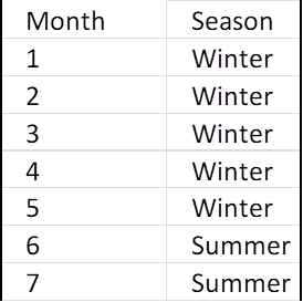
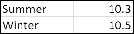
You need to determine the applicable season as the utility defines them. There will be two, Summer and Winter. Use the month column and a new supporting lookup table to populate a new Season column you will create in the master table. See screenshot below of part of the supporting table and part of the master table with the season populated.

This is where the processes diverge. First we will discuss creating a TOU analysis.
TOU-C modeling:
TOU-C analysis requires you know the weekend status of each day of the year. The master spreadsheet gives you month and date. Supplying the year of your choice create and populate a Date column using this formula:
=(DATE(2021,[@Month],[@Day]))
If you are using a table format the formula entered in the first row should automagically populate down the entire column.
Once you have the date you can create and populate a DayofWeek column with this formula: =[@DayNo].
This still does not inform your model if a given day number is a weekend day. Create and populate a column that has a 1 if the day is a weekend day:
=IF(OR([@DayNo]=1,[@DayNo]=7),1,0).
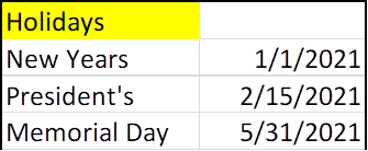
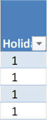
TOU-C needs to know if a given day is a holiday as recognized by the rate plan. Create a supplementary table of all holiday dates in your year of choice and using this Vlookup function, create and populate a Holiday column in which a 1 indicates it is a recognized holiday:
=COUNTIF(Holidays,[@Date])
You now have all of the information you need to determine the cost of a kilowatt hour during any given hour. You need to create supplementary table and a Vlookup key to enter that table and return a result. This key is made by concatenating the data you need. I use this suggest order: Holiday-Season-Weekend-Hour. I will include the entire supplementary table below. Here is the concatenation formula:
=CONCATENATE([@Holiday],[@Season],[@Weekend],"-",IF([@Hour]<10,0,""),C28).
Note the formula adds a leading zero to hours less than ten. Here is the result in one cell:
![]()
This tells you: Holiday, Winter, Not Weekend, Midnight (starting time)
Create two new columns where the dollar amount of the rate for that hour will go. Here is the vlookup function in first the new column:
=VLOOKUP([@Concat],E_6Matrix,7).
The second new column is:
=VLOOKUP([@Concat],E_6Matrix,8).
Here is the supplementary table below. Note there is a blank row at the end. This is needed but I don’t know quite why.
Note also that there are two rate columns. This is because this devil of a rate plan also has a tiered function built in. If you review my basic treatise on Tiered rates you know that, lacking consumption data, you are required to make an assumption to get results. If you include the high and low tier then you can calculate a range of possible values. The first new column will have the one rate, the second new column will have a different column parameter in the Vlookup and you can calculate the high and low extremes.
You now have everything you need to calculate the value of energy for every hour on each row: The amount of energy generated during that hour and the value of each kWh. Simply multiply one by the other and total the column. That was easy, wasn’t it?
E-6 tiered modeling.
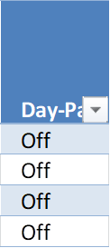
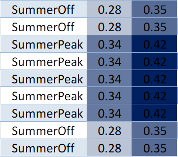
E-6 needs to know the Season and the peak/off-peak status of each hour. You already have the season. Create a supplemental table like I show partially below. Note the use of colors to help display patterns. Also shown is how this looks in the master table.
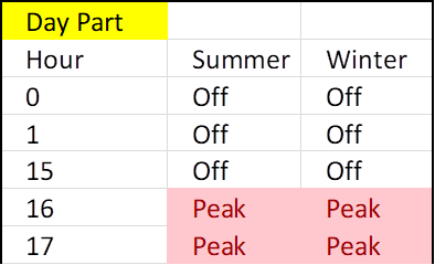
Concatenate the season and the day part to get WinterOff for example, or whatever applies.
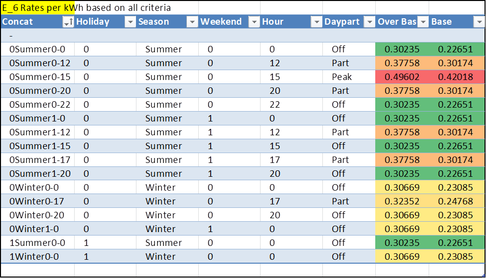
Apply a Vlookup of the table below into two new columns. One for base rates and one for over-base. Here is the supplemental table and what the master table will look like:
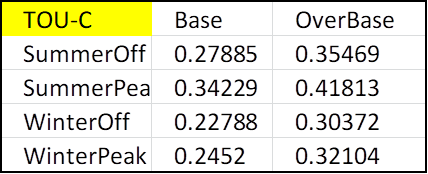
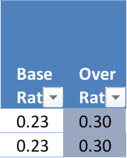
Note the master table displays only two decimal points. The rest of the fraction is there I just don’t display it. Minimize visual clutter whenever possible. The visual patterns tell you the data is behaving.
You need to apply the seasonal baseline amount. Use this Vlookup and this table:
=VLOOKUP([@Season],CRate,2)
Now the hard part: You need to determine when daily consumption exceeds the baseline value. It will happen in the middle of an hour. Start by creating and populating a column that creates a daily accumulated value of production using this formula:
=IF(B28=[@Day],M28+[@[AC System Output (kW)]],[@[AC System Output (kW)]]).
This function compares the date on the current line to the date on the previous line. If it is a new date it starts over. If not it adds this hour to the previous total. Did I mention this is the hard part?
Create and populate a column that tells you when the running total exceeds the baseline amount:
=IF([@[Daily Cumm]]<[@[Base Amnt]],1,0).
Having fun? Under returns a 1, Over returns a zero.
Create and populate a column that displays the hourly production up until the value reaches the baseline. Here is the formula. It will wrap several lines:
=IF(AND([@[Under Base]]=1,N28=1),[@[AC System Output (kW)]],IF(AND([@[Under Base]]=0,N28=1),[@[Daily Cumm]]-[@[Base Amnt]],0)).
This formula tests to see if the exceeded-base flag (Step 6 above) has just flipped. If it has not it returns the hour production. If it just flipped, it returns only the amount of hourly production that will bring the daily accumulated to the baseline ceiling. If the flag flipped in a previous line it returns zero.
Now we need to build a column that presents the amount of hourly production that exceeds the baseline:
=IF([@[Under Base]]=0,[@[AC System Output (kW)]]-Q29,0).
Now we are off to the races. Multiply the under-base hourly production by the under-base price and the same for over-base. Total the two columns and you have results for the minimum and maximum value of the energy your system will produce over a year.
Remember these three scenarios:
If you are avoiding using the higher priced over-base electricity by producing your own, the value of that homemade electricity is the higher cost you avoided.
If you are avoiding buying the lower tier electricity, the value of your power is rated at the lower price.
If you are sending excess power to the grid, my understanding it you are earning credit at the lowest rate. If you know otherwise, let me know.
Tips and tricks:
This process is complicated, or at least it is for me. Here are some tips that might help.
Use table formatting wherever possible. This provides filter and sort functions at your fingertips.
Hide or delete unnecessary columns.
Put supplementary tables on a different page. You need column and row widths to reflect what you need for the master table.
Make the width of the master spreadsheet fit within one page width. Narrow or hide columns if needed. You don’t want to be scrolling right and left.
Reduce the decimal places. Extra numbers to the right of the decimal are useful to the machine so don’t truncate or round, but display only the absolute minimum you need to establish visual patterns.
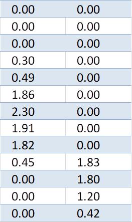
Use conditional formatting to reduce clutter. Zeros have no numerical value and they certainly have no visual value. Use custom conditional formatting to make your zeros faint or invisible. See before and after below.
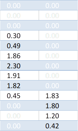
Notice the pattern revealed. The row with two non-zero values is when the daily production exceeds the E-6 baseline and the hourly production is divided between base and over-base. That pattern should repeat every day and dimming the zeros makes this pattern pop out and easy to understand.
Use conditional formatting colors to reveal patterns. Below depicts when the daypart changes. The color change is subtle but it verifies that what is supposed to be happening is happening. You don’t need to see these rate numbers but you need to know they are populating properly. The pattern tells you yes.
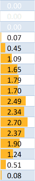
Use shapes. Below is the hourly production with conditional bar graphs. The zero values are hidden by conditional formatting. The pattern reveals itself and tells you the data is behaving predictably.
That sums up the process. Plug in our own numbers and work with this until you have the confidence to know you are making good predictions on what these rate plans will do to you or your client’s bottom line. See the above URL for example spreadsheets.
You have my permission to share this information but make sure any representation includes the following:
Courtesy of Miller Solar
Sincerely,
William Miller